Our previously described experiment demonstrates how standard neural network architectures fail to obtain decent classification accuracy and loss when working with image datasets that exhibit similarities between different tissue structures, noise, and other imaging artifacts.

Essentially, it’s hard for networks to learn a rich set of discriminative features, so consequently, they are failing to classify pathologies for unknown ACL contexts. That finally led us to conclude that we might be able to yield better results if the dataset is previously subjected to highly demanding segmentation of each recording. In the following paragraphs, we’ll briefly outline the solution we developed and tested.

Due to different approaches to taking MR images (different recording techniques, space between images), volumes need to be preprocessed first. We implemented a preprocessing technique using the MRNet architecture that enables better classification of ACL in knee joint MR images. Our preprocessing process is two-fold:

1. Volume preprocessing
2. Slice preprocessing

Volume preprocessing

Volume preprocessing represents the reduction of the number of images within a volume to a given number K. As the number of images in a volume differs in our datasets, the idea is to find K representatives that represent the volume well. We performed the dimensionality reduction via the non-negative matrix factorization method (NMF) and found ten (K = 10) base images within each volume. The idea behind this method is to display each image of the original volume as a non-negative superposition of K base images:

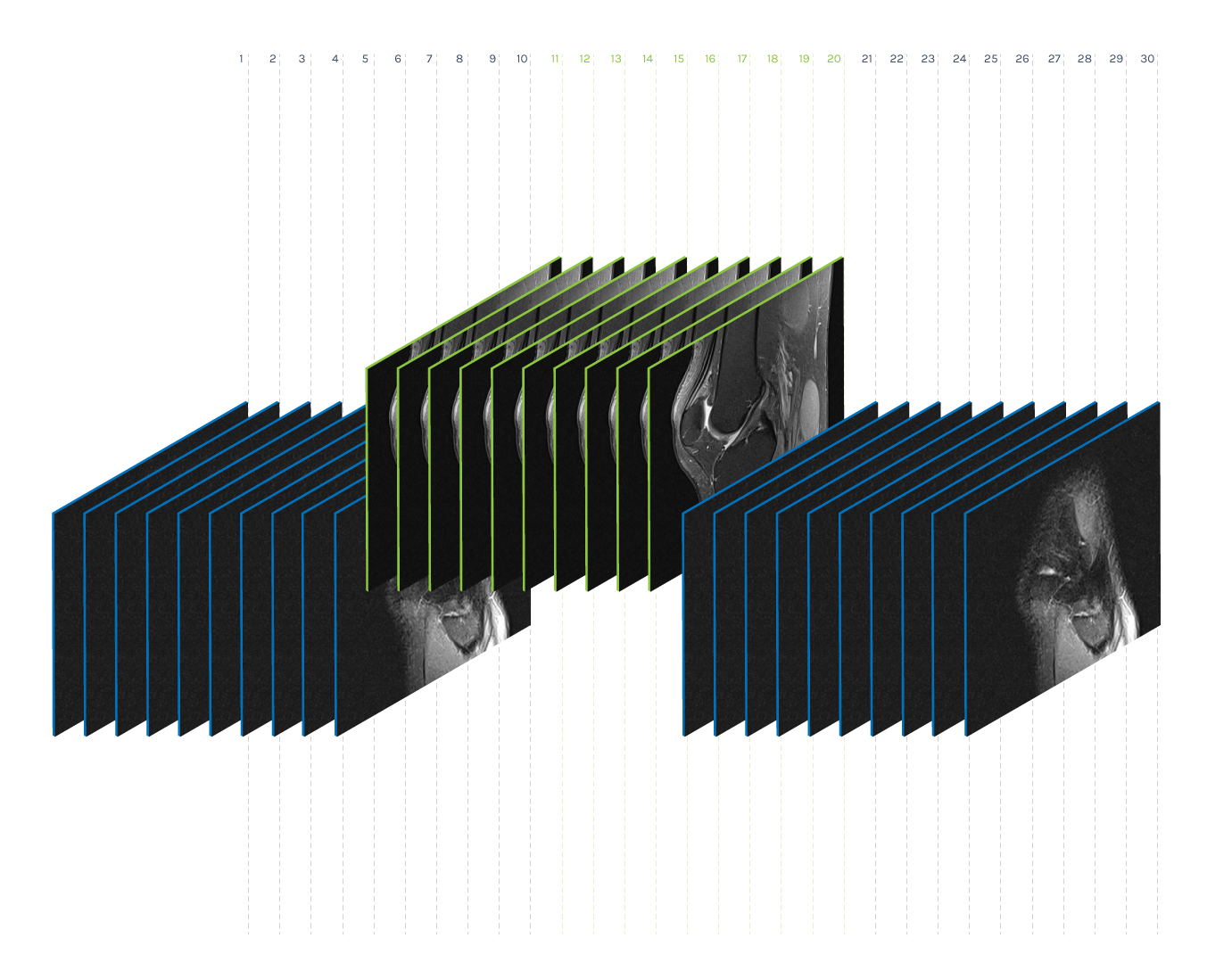
Preprocessing of volume (K = 10)

Slice preprocessing

Slice preprocessing uses volume reduction smoothing and a standard histogram pixel intensity normalizer to reduce the appearance of artifacts. Using automatic thresholding, the foreground mask (FG mask) was then defined to include all pixels representing the knee except for the background. The output of this step is a set of foreground pixels per slice:

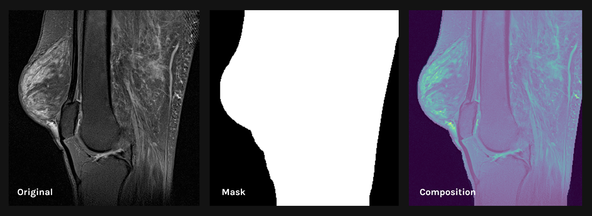
Original slice (left), the foreground mask (middle) and preprocessed slice (right)

Segmentation

The points of interest within the slice are specific pixel intensities and depend on the recording technique. To locate pixels containing information of interest, a semi-automated pixel segmentation process was conducted as follows:

1. Preprocessed slices were fed to the segmentation process, which uses the K-Means algorithm to cluster similar pixels by intensities. For clustering needs, we used the K-Means algorithm with parameter K = 20.
2. The clusters were then sorted according to intensities.
3. The start and end numbers of the clusters we want to use are meta-parameters, and in our case, we determined them depending on the MRI volume recording technique. We experimented with results and found out that, in most volumes, it was sufficient to select the first four clusters, which, as a rule, represented all the pixels of the FG mask that had the dominant four shades of color (darker regions). All other pixels were omitted since only these regions contained information about the anatomical artifact.

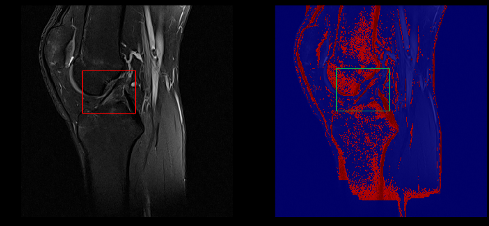
Example of healthy ACL visible in a sagittal slice (left) captured in our segmentation (right)

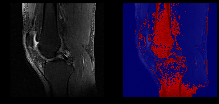
ACL lesion (left) captured in our segmentation (right)

The segmentation process has two essential advantages:

• Convolutional neural networks are fed with structured data which helps them to isolate key features easier and accurately without requiring manual segmentation on training data;
• “Sparsification” of the input signal that opens the door to alternative methods specializing in a rare input signal.

With data preprocessing and segmentation in place, we obtained our best AUC thus far: from 0.88 to 0.90, depending on the evaluation dataset. Furthermore, as in the previous experiments, during the evaluation process, we observed the network’s behavior using Class Activation Maps (CAM - the images below). We obtained various feature maps by propagating the knee images through the network and stopping at different target layers. By doing so, we noticed that sometimes the network was picking up on other underlying patterns similar in texture (veins, knee effusions, etc.), and not just structures indicative of the certain ACL condition.

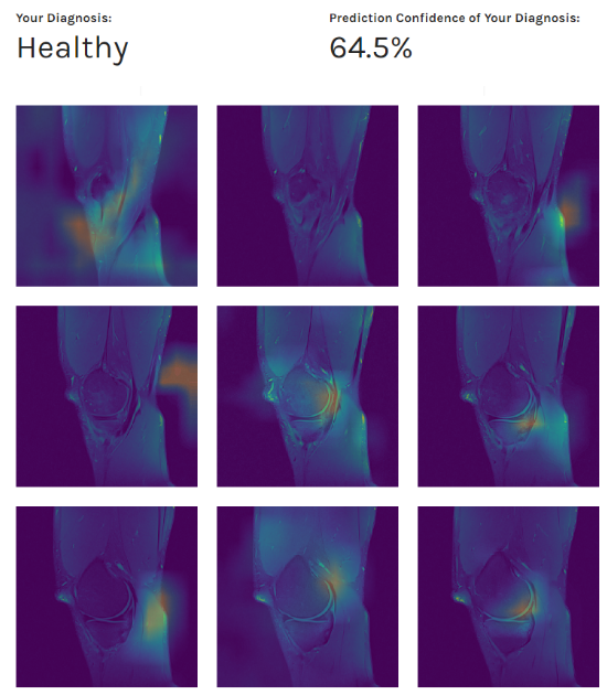
Patient’s diagnosis (above) and MRI scans preview combined with our class activation mapping (below)

Results obtained led us to conclusion that features learned by the network perform well as generic features and can identify only to some extent the discriminative image regions used for categorization.

Conclusion

Developing a robust segmentation process proved to be the key piece in creating a deep learning model capable of picking out discriminative features of the ACL joint. This further improved the accuracy of the model and gave us confidence that the features it captures are actually relevant for giving an accurate diagnosis.

The model is still lacking - mostly related to the generalization of its features, but we consider the results to be a solid success. Its accuracy can likely be further improved by obtaining a more balanced dataset, deepening the network, training from scratch, or being more aggressive with network analysis.

In the next blog post we will explore how image preprocessing and segmentation look in code.